My First Convolutional Neural Network : Fashion MNIST
실습목표
- CNN의 기본 아이디어를 안다.
- CNN의 구조를 그리고, 코드로 옮길 수 있다.
Keras Upgrade
!pip install keras-nightlyRequirement already satisfied: keras-nightly in /usr/local/lib/python3.10/dist-packages (3.6.0.dev2024101603)
Requirement already satisfied: absl-py in /usr/local/lib/python3.10/dist-packages (from keras-nightly) (1.4.0)
Requirement already satisfied: numpy in /usr/local/lib/python3.10/dist-packages (from keras-nightly) (1.26.4)
Requirement already satisfied: rich in /usr/local/lib/python3.10/dist-packages (from keras-nightly) (13.9.2)
Requirement already satisfied: namex in /usr/local/lib/python3.10/dist-packages (from keras-nightly) (0.0.8)
Requirement already satisfied: h5py in /usr/local/lib/python3.10/dist-packages (from keras-nightly) (3.11.0)
Requirement already satisfied: optree in /usr/local/lib/python3.10/dist-packages (from keras-nightly) (0.13.0)
Requirement already satisfied: ml-dtypes in /usr/local/lib/python3.10/dist-packages (from keras-nightly) (0.4.1)
Requirement already satisfied: packaging in /usr/local/lib/python3.10/dist-packages (from keras-nightly) (24.1)
Requirement already satisfied: typing-extensions>=4.5.0 in /usr/local/lib/python3.10/dist-packages (from optree->keras-nightly) (4.12.2)
Requirement already satisfied: markdown-it-py>=2.2.0 in /usr/local/lib/python3.10/dist-packages (from rich->keras-nightly) (3.0.0)
Requirement already satisfied: pygments<3.0.0,>=2.13.0 in /usr/local/lib/python3.10/dist-packages (from rich->keras-nightly) (2.18.0)
Requirement already satisfied: mdurl~=0.1 in /usr/local/lib/python3.10/dist-packages (from markdown-it-py>=2.2.0->rich->keras-nightly) (0.1.2)Real Game : CNN on Fashion MNIST
여기에서는 여러분이 직접 코드를 완성해야 하는 문제가 곳곳에 있습니다!
'''
라이브러리들을 불러오자.
'''
import numpy as np
import pandas as pd
import matplotlib.pyplot as plt

import random as rd
from sklearn.metrics import accuracy_score

import keras
Data Loading
(train_x, train_y), (test_x, test_y) = keras.datasets.fashion_mnist.load_data()print(train_x.shape, train_y.shape, test_x.shape, test_y.shape)(60000, 28, 28) (60000,) (10000, 28, 28) (10000,)labels = ["T-shirt/top", # index 0
"Trouser", # index 1
"Pullover", # index 2
"Dress", # index 3
"Coat", # index 4
"Sandal", # index 5
"Shirt", # index 6
"Sneaker", # index 7
"Bag", # index 8
"Ankle boot"] # index 9
print(labels)['T-shirt/top', 'Trouser', 'Pullover', 'Dress', 'Coat', 'Sandal', 'Shirt', 'Sneaker', 'Bag', 'Ankle boot']'''
Ctrl+Enter를 이용하여
반복 실행 해보자!
'''
id = rd.randrange(0,10000)
print(f'id = {id}')
print(f'다음 그림은 {labels[test_y[id]]} 입니다.')
plt.imshow(test_x[id], cmap='gray')
plt.show()
X : Min-Max Scaling
- 최소값 0, 최대값 1로 통일하는 스케일링
train_x.min(), train_x.max()

train_x = (train_x - train_x.min()) / (train_x.max() - train_x.min())
test_x = (test_x - test_x.min()) / (test_x.max() - test_x.min())

train_x.min(), train_x.max()
(0.0, 1.0)X : Reshape(# of data, 28, 28, 1)
- 끝에 1을 달아서 그레이스케일(흑백)을 명시해준다.
train_x.shape, test_x.shape((60000, 28, 28), (10000, 28, 28))train_x = train_x.reshape(train_x.shape[0],28,28,1)
test_x = test_x.reshape(test_x.shape[0],28,28,1)
train_x.shape, test_x.shape((60000, 28, 28, 1), (10000, 28, 28, 1))Y : One-Hot Encoding
len(np.unique(train_y))

from keras.utils import to_categorical, plot_model
train_y = to_categorical(train_y,10)
test_y = to_categorical(test_y,10)
len(np.unique(train_y)), train_y.shape, test_y.shape(2, (60000, 10), (10000, 10))코드를 완성해주세요!
- 자유롭게 먼저 해보는 것을 추천
- 구조를 따라서 코딩을 한다면..
- 인풋 레이어
- Convolution : 필터수 32개, 사이즈(3, 3), same padding
- BatchNormalization
- Convolution : 필터수 32개, 사이즈(3, 3), same padding
- BatchNormalization
- MaxPooling : 사이즈(2,2) 스트라이드(2,2)
- DropOut : 25% 비활성화
- Convolution : 필터수 64개, 사이즈(3, 3), same padding
- BatchNormalization
- Convolution : 필터수 64개, 사이즈(3, 3), same padding
- BatchNormalization
- MaxPooling : 사이즈(2,2) 스트라이드(2,2)
- DropOut : 25% 비활성화
- Flatten
- Fully Connected Layer : 노드 512개
- BatchNormalization
- 아웃풋 레이어
# 1. 세션 클리어
keras.utils.clear_session()

# 2. 모델 선언
model = keras.models.Sequential()

# 3. 레이어 조립
model.add( keras.layers.Input(shape=(28,28,1)) )

model.add( keras.layers.Conv2D(filters=32,        # 새롭게 제작하려는 feature map의 수! - 서로 다른 필터 32개 사용하겠다.
                               kernel_size=(3,3), # Conv2D Layer filter의 가로세로 사이즈 (depth는 케라스가 보정!)
                               strides=(1,1),     # Conv2D Layer filter의 이동 보폭
                               padding='same',    # 앞전 feature map의 가로세로 사이즈 유지 | 외곽 정보 더 반영
                               activation='relu', # 빼먹지 않기!
                               ) )
model.add( keras.layers.BatchNormalization() )

model.add( keras.layers.Conv2D(filters=32,        # 새롭게 제작하려는 feature map의 수!
                               kernel_size=(3,3), # Conv2D Layer filter의 가로세로 사이즈 (depth는 케라스가 보정!)
                               strides=(1,1),     # Conv2D Layer filter의 이동 보폭
                               padding='same',    # 앞전 feature map의 가로세로 사이즈 유지 | 외곽 정보 더 반영
                               activation='relu', # 빼먹지 않기!
                               ) )
model.add( keras.layers.BatchNormalization() )

model.add( keras.layers.MaxPool2D(pool_size=(2,2), # Maxpooling layer filter의 가로세로 사이즈
                                  strides=(2,2),   # Maxpooling layer filter의 이동 보폭
                                  ) )
model.add( keras.layers.Dropout(0.25) )

model.add( keras.layers.Conv2D(filters=64,        # 새롭게 제작하려는 feature map의 수!
                               kernel_size=(3,3), # Conv2D Layer filter의 가로세로 사이즈 (depth는 케라스가 보정!)
                               strides=(1,1),     # Conv2D Layer filter의 이동 보폭
                               padding='same',    # 앞전 feature map의 가로세로 사이즈 유지 | 외곽 정보 더 반영
                               activation='relu', # 빼먹지 않기!
                               ) )
model.add( keras.layers.BatchNormalization() )

model.add( keras.layers.MaxPool2D(pool_size=(2,2), # Maxpooling layer filter의 가로세로 사이즈
                                  strides=(2,2),   # Maxpooling layer filter의 이동 보폭
                                  ) )
model.add( keras.layers.Dropout(0.25) )

model.add( keras.layers.Flatten() )
model.add( keras.layers.Dense(512, activation='relu') )
model.add( keras.layers.Dense(10, activation='softmax') )


model.summary()
Early Stopping을 활용한 학습
- 조건
- validation_split = 0.2
- 1 epochs만 관찰해가며 속도가 가장 빠른 batch_size 찾아보기. 128개부터 시작하여 조절해볼 것.
- EarlyStopping. val_loss가 5 epoch 전과 비교하여 개선되지 않으면 스탑
- 이미지 시각화를 위해 hist 변수에 학습 과정을 넣어주세요.
from keras.callbacks import EarlyStopping# 파라미터 시각화
plot_model(model,
show_shapes=True,
show_layer_activations=True,
show_trainable=True,
)
# 이미지 용량이 매우 커서 블로그에 올라가지 않음. 실습은 따로 해보시길 바랍니다.es = EarlyStopping(monitor='val_loss', # 얼리스토핑을 적용할 관측 지표
min_delta=0, # 임계값. monitor에서 지정한 지표가 min_delta의 값보다 크게 변해야 성능 개선으로 간주
patience=5, # 성능 개선이 발생하지 않을 때, 얼마나 더 지켜볼 것인지.
verbose=1, # 얼리스토핑 적용 문구
restore_best_weights=True,# 최적의 가중치를 가진 epoch 시점으로 되돌림!
)model.compile(optimizer='adam', loss='categorical_crossentropy',metrics=['accuracy'])
hist = model.fit(train_x, train_y, validation_split=0.2, verbose=1, epochs=1000, callbacks=[es])Epoch 1/1000
1500/1500 ━━━━━━━━━━━━━━━━━━━━ 25s 7ms/step - accuracy: 0.8040 - loss: 0.6562 - val_accuracy: 0.9006 - val_loss: 0.2761
Epoch 2/1000
1500/1500 ━━━━━━━━━━━━━━━━━━━━ 7s 5ms/step - accuracy: 0.9013 - loss: 0.2695 - val_accuracy: 0.8972 - val_loss: 0.2827
Epoch 3/1000
1500/1500 ━━━━━━━━━━━━━━━━━━━━ 9s 4ms/step - accuracy: 0.9140 - loss: 0.2340 - val_accuracy: 0.9147 - val_loss: 0.2368
Epoch 4/1000
1500/1500 ━━━━━━━━━━━━━━━━━━━━ 6s 4ms/step - accuracy: 0.9249 - loss: 0.2044 - val_accuracy: 0.9252 - val_loss: 0.2192
Epoch 5/1000
1500/1500 ━━━━━━━━━━━━━━━━━━━━ 6s 4ms/step - accuracy: 0.9353 - loss: 0.1728 - val_accuracy: 0.9221 - val_loss: 0.2305
Epoch 6/1000
1500/1500 ━━━━━━━━━━━━━━━━━━━━ 6s 4ms/step - accuracy: 0.9392 - loss: 0.1637 - val_accuracy: 0.9222 - val_loss: 0.2202
Epoch 7/1000
1500/1500 ━━━━━━━━━━━━━━━━━━━━ 6s 4ms/step - accuracy: 0.9456 - loss: 0.1471 - val_accuracy: 0.9253 - val_loss: 0.2187
Epoch 8/1000
1500/1500 ━━━━━━━━━━━━━━━━━━━━ 7s 4ms/step - accuracy: 0.9539 - loss: 0.1251 - val_accuracy: 0.9272 - val_loss: 0.2147
Epoch 9/1000
1500/1500 ━━━━━━━━━━━━━━━━━━━━ 10s 4ms/step - accuracy: 0.9577 - loss: 0.1137 - val_accuracy: 0.9252 - val_loss: 0.2378
Epoch 10/1000
1500/1500 ━━━━━━━━━━━━━━━━━━━━ 6s 4ms/step - accuracy: 0.9639 - loss: 0.0997 - val_accuracy: 0.9272 - val_loss: 0.2359
Epoch 11/1000
1500/1500 ━━━━━━━━━━━━━━━━━━━━ 6s 4ms/step - accuracy: 0.9671 - loss: 0.0890 - val_accuracy: 0.9316 - val_loss: 0.2592
Epoch 12/1000
1500/1500 ━━━━━━━━━━━━━━━━━━━━ 6s 4ms/step - accuracy: 0.9701 - loss: 0.0787 - val_accuracy: 0.9316 - val_loss: 0.2499
Epoch 13/1000
1500/1500 ━━━━━━━━━━━━━━━━━━━━ 10s 4ms/step - accuracy: 0.9712 - loss: 0.0775 - val_accuracy: 0.9307 - val_loss: 0.2352
Epoch 13: early stopping
Restoring model weights from the end of the best epoch: 8.이미지 시각화
plt.figure(figsize=(10, 5))
plt.plot(hist.history['accuracy'])
plt.plot(hist.history['val_accuracy'])
plt.title('Accuracy : Training vs Validation')
plt.ylabel('Accuracy')
plt.xlabel('Epoch')
plt.legend(['Training', 'Validation'], loc=0)
plt.show()
plt.figure(figsize=(10, 5))
plt.plot(hist.history['loss'])
plt.plot(hist.history['val_loss'])
plt.title('Loss : Training vs Validation')
plt.ylabel('Loss')
plt.xlabel('Epoch')
plt.legend(['Training', 'Validation'], loc=0)
plt.show()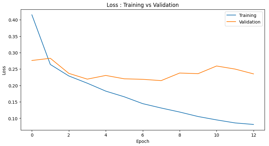
y_pred = model.predict(test_x)
y_pred.shape
313/313 ━━━━━━━━━━━━━━━━━━━━ 1s 2ms/step(10000, 10)single_y_pred = y_pred.argmax(axis=1)
single_y_pred.shape(10000,)print(test_y.shape)
single_test_y = test_y.argmax(axis=1)
print(single_test_y.shape)(10000, 10)
(10000,)test_acc = accuracy_score(single_test_y, single_y_pred)
print(f'테스트셋 정확도 : {test_acc*100:.2f}%' )테스트셋 정확도 : 92.11%'''
성능 확인을 위해
Ctrl+Enter를 이용하여
반복 실행 해보자!
'''
id = rd.randrange(0,10000)
print(f'id = {id}')
print(f'다음 그림은 숫자 {labels[single_test_y[id]]} 입니다.')
print(f'모델의 예측 : {labels[single_y_pred[id]]}')
print(f'모델의 카테고리별 확률 : {np.floor(y_pred[id]*100)}')
if single_test_y[id] == single_y_pred[id] :
print('정답입니다')
else :
print('틀렸어요')
plt.imshow(test_x[id].reshape([28,-1]), cmap='gray')
plt.show()
'''
틀린 것만 관찰해보자!

Ctrl+Enter를 이용하여
반복 실행 해보자!
'''

true_false = (single_test_y==single_y_pred)
f_id = np.where(true_false==False)[0]        # 틀린 것들의 인덱스 반환
f_n = len(f_id)                              # 틀린 것들이 총 몇 개나 될까?

id = f_id[rd.randrange(0,f_n)]

print(f'id = {id}')
print(f'다음 그림은 숫자 {labels[single_test_y[id]]} 입니다.')
print(f'모델의 예측 : {labels[single_y_pred[id]]}')
print(f'모델의 카테고리별 확률 : {np.floor(y_pred[id]*100)}')

if single_test_y[id] == single_y_pred[id] :
    print('정답입니다')
else :
    print('틀렸어요')

plt.imshow(test_x[id].reshape([28,-1]), cmap='gray')
plt.show()
'AI_딥 러닝_시각지능' 카테고리의 다른 글
| AI_파이썬_시각지능_CNN_Image_SmallData2024 (0) | 2024.12.30 |
|---|---|
| AI_파이썬_시각지능_CNN_exercise_notMNIST_small_2024 (0) | 2024.12.30 |
| AI_파이썬_시각지능_CNN_exercise_CIFAR10_2024 (1) | 2024.12.30 |
| AI_파이썬_시각지능_CNN_2024 (0) | 2024.12.30 |
| AI_파이썬_시각지능_notMNIST_small_2024 (0) | 2024.12.30 |


